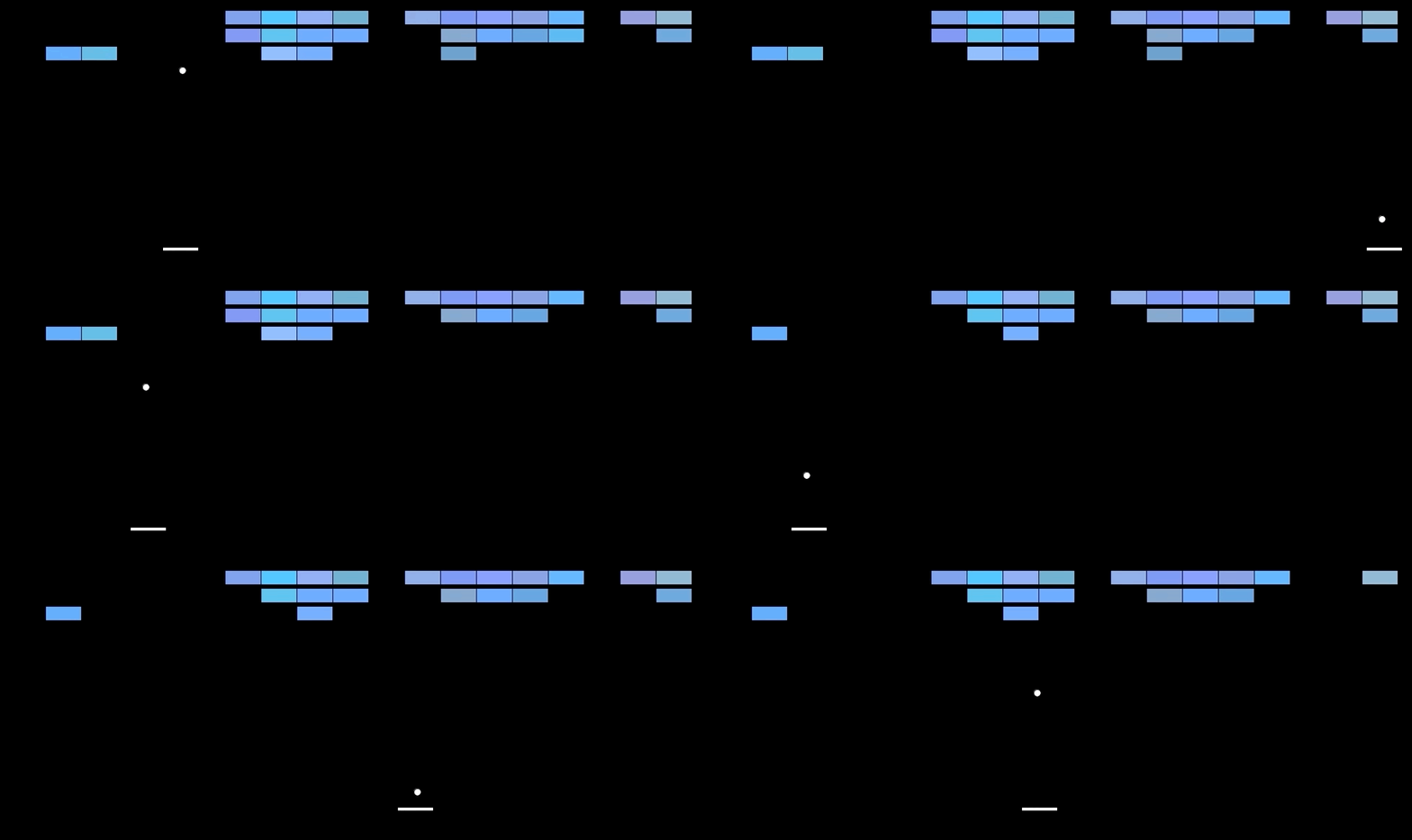
Hello there! ✋ This week we explore how Deep learning (DL) can be combined with Reinforcement learning (RL) to teach AI agent to play selection of Atari 2600 games. We’ll delve into DeepMinds’ groundbreaking classic, “Playing Atari with Deep Reinforcement Learning” (2013), which not only represents the first successfull application of Deep Learning to RL, but also shows that the trained agent outperformed state-of-the-art (SOTA) methods and partly even humans in some of the ATARI games such as Breakout. 👇 (gif from here)
Playing Atari games with Deep RL 🕹️
📍 Context. In 2013, one of the major challenges in the field of RL was to control agents based on high dimensional inputs such as video or speech. Fortunately, around the same time, DL architectures such as Convovolutional or Reccurent neural networks (CNN, RNN), proved to be SOTA methods for problems like image classification, object detection and speech recognition. This led the researchers from DeepMind to the idea of combining advances in DL with the RL. Their model, called Deep-Q-Network (DQN), learned purely from pixel input to play seven Atari games and outperformed even baselines that utilize heavily hand-crafted and fine-tuned features. The paper set the basis for the entire field of deep reinforcement learning and established DeepMind as one of the leading AI companies in the world.
🤖 Reinforcement learning. Reinforcement Learning (RL) is a machine learning training method that rewards desired behaviours and/or punishes undesired ones. In a typical setting, an agent interacts with an environment. The agent can perform actions to influence the environment and, in return, receives a state (e.g. next frame in the game) and a reward - a scalar value indicating whether the action was good or bad. The central task is then to find actions that maximise the total reward the agent can obtain. One way to learn how to choose the most optimal action given the current state is through Q-Learning, which we will explain in a second.
To provide a concrete example, let’s consider the Breakout game. In this game, the agent must determine where to move the paddle so that it hits the ball, which then destroys one of the bricks. The ultimate goal of the agent is to destroy all the bricks, which would result in the maximum possible score/reward. To achieve this goal, the agent must learn not just the most optimal immediate action, but rather the action that will maximize the overall score at the end of the game. To see the agent’s learning progress, you can watch a 2 minute video of Breakout being played.
🇶 Q-Learning. Instead of getting into all the low-level details, including the math, which is very well described in this video, let’s focus on describing the conceptual idea. Q-learning is based on a Q-function which takes state and action as input and outputs the total reward based on these two inputs.
To provide a practical example, imagine it’s a Friday night and you’re trying to decide whether to go out and enjoy life, or stay home, watch Drive to Survive on Netflix, and avoid a hangover the next day. This decision may or may not affect future decisions, like if you decide to work on your thesis or just sleep. The reward is the level of happiness each day. When your life comes to an end, you obtain a total reward which is the sum of all rewards for each day in your life from the moment you took the decision. Naturally, you will choose the action that maximizes the total reward. The question is, how do we get to this magical Q-function?
🔦 Searching for the Q-function. To approximate the Q-function, we use a Neural Network, or what the paper calls a Deep Q-Network (DQN). Details of this network are described in the subsequent architecture section. For now, all you need to know is that the network takes the previously seen four video frames as input and outputs an estimate of the total reward for each possible next action.
The more important question, however, is how we teach the network to output correct estimates. In Deep Learning, there is always some input and corresponding ground truth output. In the case of the Q-function, the goal is to find out whether its estimate of the total reward for the chosen action (the one with the maximum total reward) was good or completely off. For this reason, every time the agent makes a transition from one state to another, the information about the transition is saved in the so-called experience replay buffer (think database with limited memory), which is then used for training the network as described below.
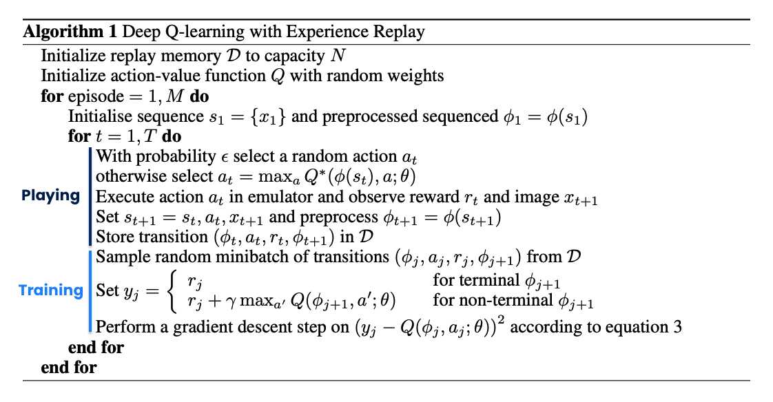
📈 Training algorithm. After storing the transition (sample) in the replay buffer, the algorithm randomly selects a minibatch of samples from the buffer. Each sample includes the following information: the previous state, the action taken, the immediate reward for the action taken, and the next state to which the action led. In a second, we will explain how these are used. Now, recall that in DL, you feed the model with some input, take its output yhat, and compare it to the ground truth value y. For instance, in regression, you take the difference between the two values and square it. This results in a loss that is then used to update the model’s weights via backpropagation.
Going back to our sample from the replay buffer, the question is, what is yhat in this case, and what is the corresponding y? Let’s start with the prediction yhat. We feed our DQN (representing the Q-function) with the previous state and select the total reward that corresponds to the action taken. The ground truth value y is then the sum of the reward obtained and the total reward estimate produced by a target DQN based on the next state. Target DQN is simply a copy of the trained DQN. The copy is made every C updates. This technique helps to stabilize the training and prevent the Q-network from overestimating the Q-values. Finally, the figure below puts nicely all things together and should give you idea how all the pieces described fit together.
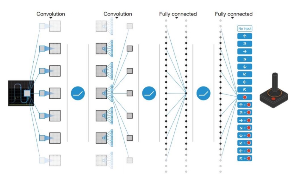
🏗️ Model architecture. The DQN architecture is surprisingly simple by today’s standards. It takes an 84 × 84 × 4 image produced by a preprocessing function, which involves downsampling, cropping, grayscale conversion, and stacking 4 frames. The image is then fed through two convolutional and two linear layers with ReLU’s in between. The number of output neurons corresponds to the number of valid actions, which varies between 4 and 18 for the evaluated corpus of games (Figure adapted from here).
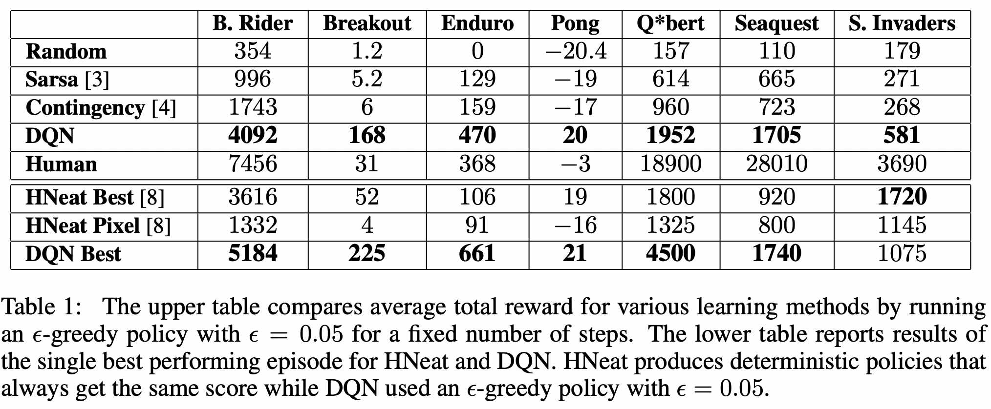
🤯 Results. The model outperforms SOTA methods on 6 out of 7 games tested. (the bottom table) Further, it can even beat human players in three of them. (upper table) This is especially impressive considering that previous SOTA approaches used highly game-specific information to make predictions, while the Deep Q Network learns from nothing but the pixel input. Notably, humans are superior to the model in games that have a longer playing time. Intuitively, this makes sense, given that the core task of the network is to approximate the Q function that returns the estimated reward until the end of the game, which becomes more difficult with increasing game length.
🔮 Key Takeaways
😍 DL in RL! The paper demonstrated that it is possible to combine deep learning with reinforcement learning and achieve SOTA performance for the selected task. Further, the paper opened doors for subsequent research exploring other possible applications, as well as improving the learning procedure.
🔄 Experience replay. The replay buffer technique helps to break up the correlations between consecutive samples and leads to more stable training. This innovation was extremely important for the combination of DL to the RL.
🧠 Simplicity. In today’s world where models can have billions of parameters, it is good to remind ourselves that even small models can produce impressive results.
📣 Stay in touch
That’s it for this week. We hope you enjoyed reading this post. 😊 To stay updated about our activities, make sure you give us a follow on LinkedIn and Subscribe to our Newsletter. Any questions or ideas for talks, collaboration, etc.? Drop us a message at hello@aitu.group.
